Working with HDF5 files

Caterva2 offers native support for working with HDF5 files. See here for a video demonstration. The notebook used is available on github. In this tutorial, we will cover the same material: This tutorial demonstrates how to use the Cat2Cloud system with large HDF5 files. You’ll learn how to upload, access, manipulate, and visualize HDF5 data both through proxy objects and Blosc2 arrays using the Caterva2 Python client.

What is an HDF5 file?

HDF stands for Hierarchical Data Format. HDF5 is a file format and set of tools for managing complex data. It is designed to store and organize large amounts of heterogeneous data, enabling quick access and efficient storage, using compression for example. HDF5 files are made up of a root (/) which may then contain the file contents. These contents are organised using the two main structures of HDF5 files - groups (which are like subdirectories) and datasets. Both datasets and groups possess metadata, which may include special, bespoke information about the object in the form of attributes (attrs).

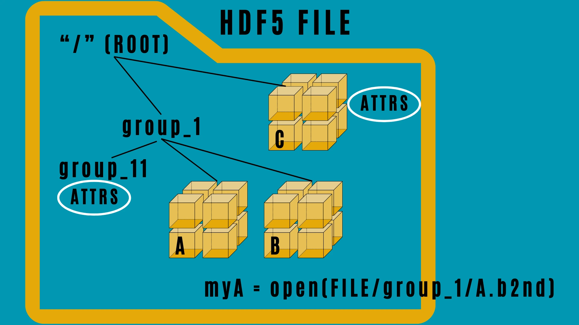
Schematic of hdf5 file structure

Loading a HDF5 file

HDF5 files are common in many scientific and industrial applications, and so examples abound online. We’re going to use some example diffraction data from a synchrotron, provided by the silx project. This may be downloaded locally (after importing necessary libraries - see the notebook mentioned at the beginning of this tutorial):

dir_path = "kevlar"
if not os.path.exists(f"{dir_path}.h5"):
    response = requests.get("http://www.silx.
        org/pub/pyFAI/pyFAI_UM_2020/data_ID13
        /kevlar.h5")
    with open(f"{dir_path}.h5", "wb") as file:
        file.write(response.content)

Unfolding the file

In order to handle the .h5 file using Cat2Cloud, we must expose the hierarchical structure of the HDF5 file on the server, which in our case will be the demo server at https://cat2.cloud/demo. This is done by uploading the file to the Caterva2 server and then unfolding it, using a memory-light structure of subdirectories and proxy datasets.

url = "https://cat2.cloud/demo"
client = cat2.Client(url,
                    ("user@example.com", "foobar11"))
myroot = client.get("@shared")
print(f"Before uploading and unfolding:
        {myroot.file_list}")
local_address = f"{dir_path}.h5"
remote_address = myroot.name + "/" + local_address
apath = client.upload(local_address, remote_address)
bloscpath = client.unfold(apath)

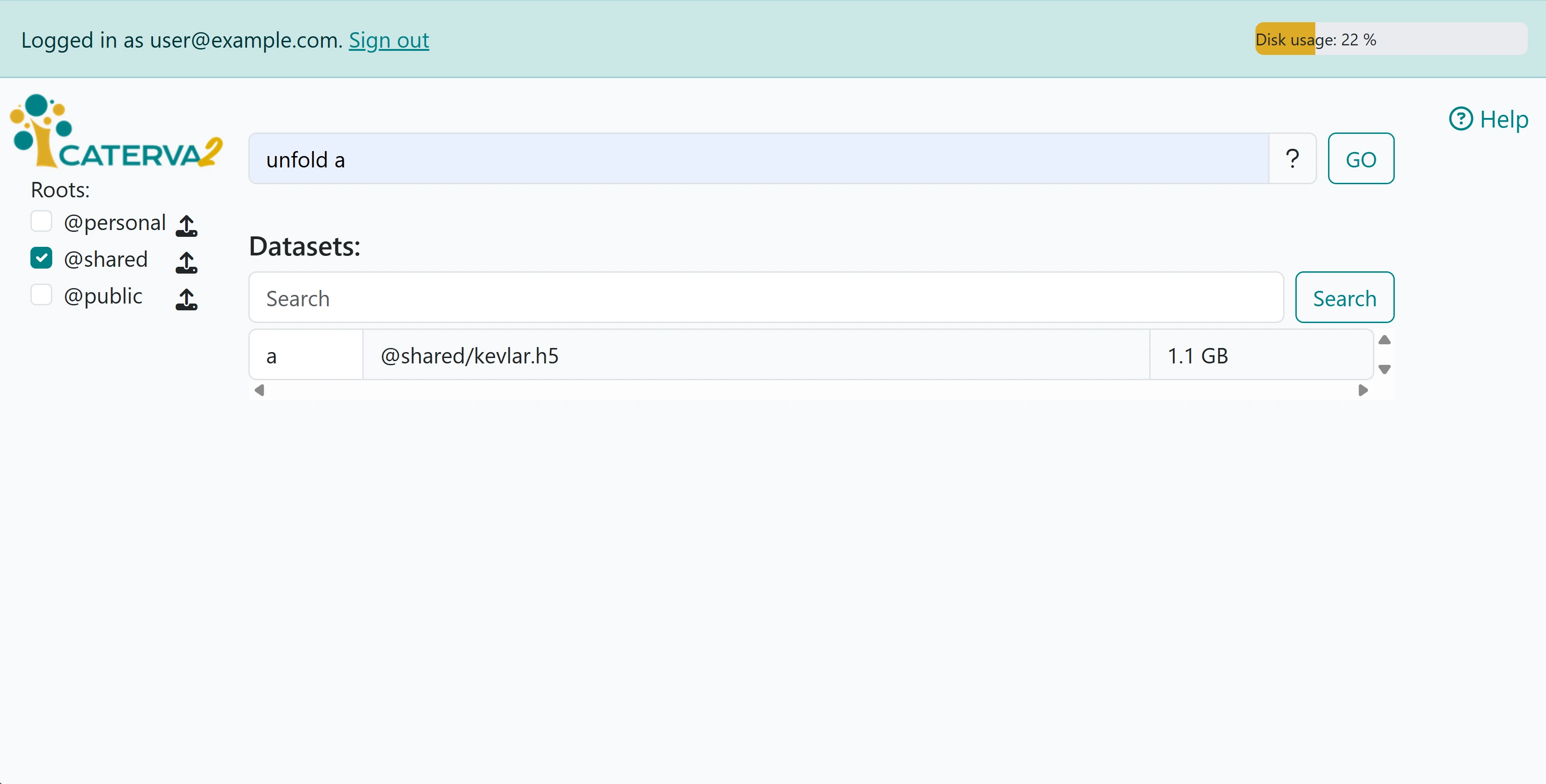
By running the line print(f"After uploading and unfolding: {myroot.file_list}"), one can check that the .h5 indeed has been correctly exposed. Note that one may also use the unfold command in the prompt on the web client, applying it to the uploaded file:

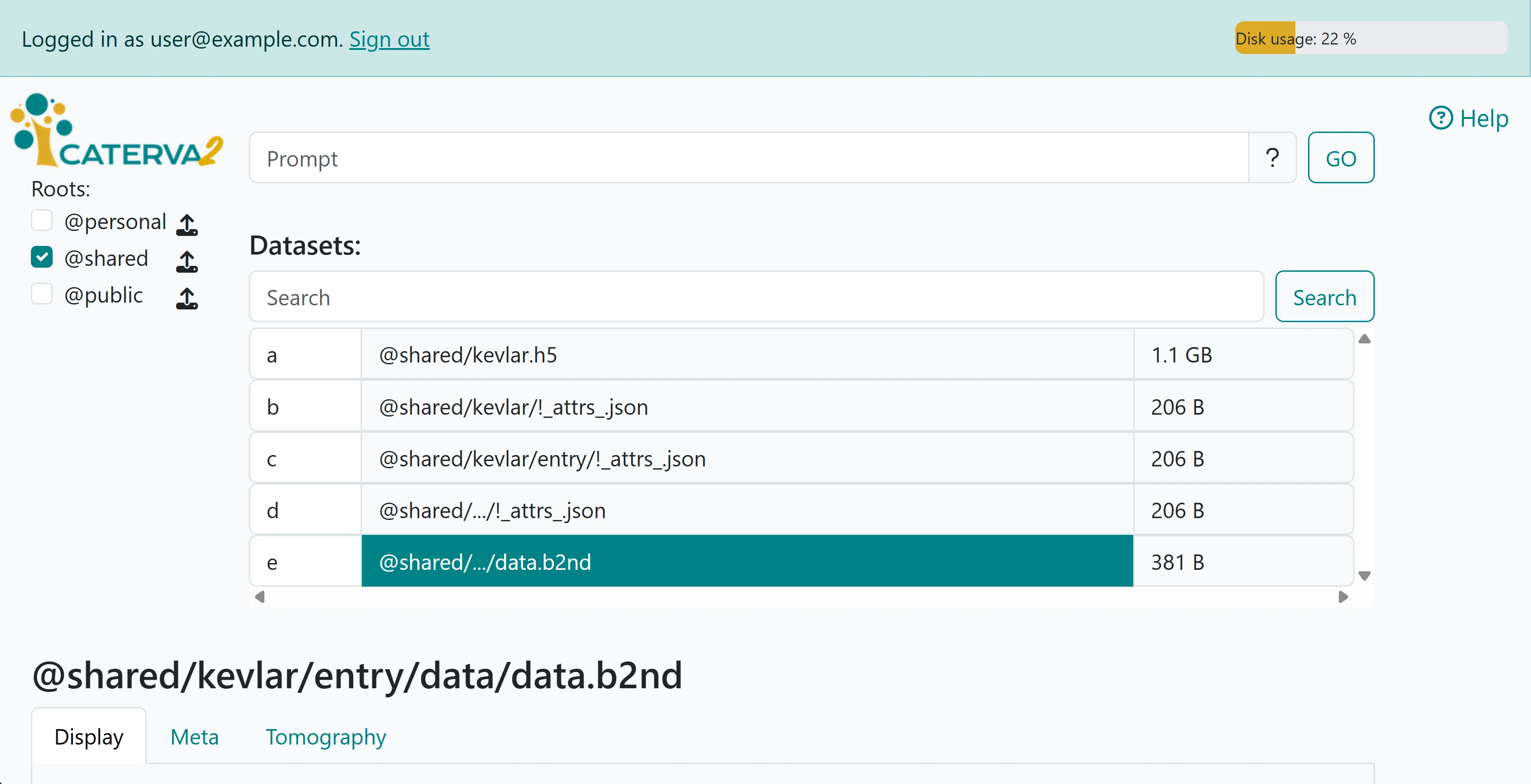
The unfolded file structure is clearly visible in the second image. We may now perform operations on the `.b2nd` proxy.

Examining the unfolded data

We can define a local reference which points to the data on the server (specifically the proxy), and we can obtain the easily obtain some of the data and plot it like so:

proxy = myroot["kevlar/entry/data/data.b2nd"]
cmap = plt.cm.viridis
example_image = proxy[5]
fig = plt.figure()
plt.imshow(example_image / 65535,
           figure=fig, cmap=cmap, vmax=1, vmin=0)

First visualisation

As is clear, not much detail can be seen in the image; this is due to outlier pixels maxing out the image range. We can use a lazyexpr to apply a function to the data, which will be executed on the server side, and then we can visualise the result. The following code applies a conditional expression to the data, increasing the signal pixels.

image = client.lazyexpr("expr",
                        "where(a < 10, a * 32000, a)",
                         {"a": proxy.path})
example_image = client.get(image)[5] / 65535
fig = plt.figure()
plt.imshow(example_image, figure=fig,
            cmap=cmap, vmax=1, vmin=0)

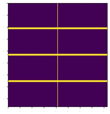
The result is an image with the desired diffraction pattern visible, as shown below:

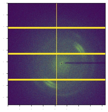
Second visualisation

We can also go to the web client and directly visualize the lazy expression we have just generated and saved via the Tomography tab for the saved expression:

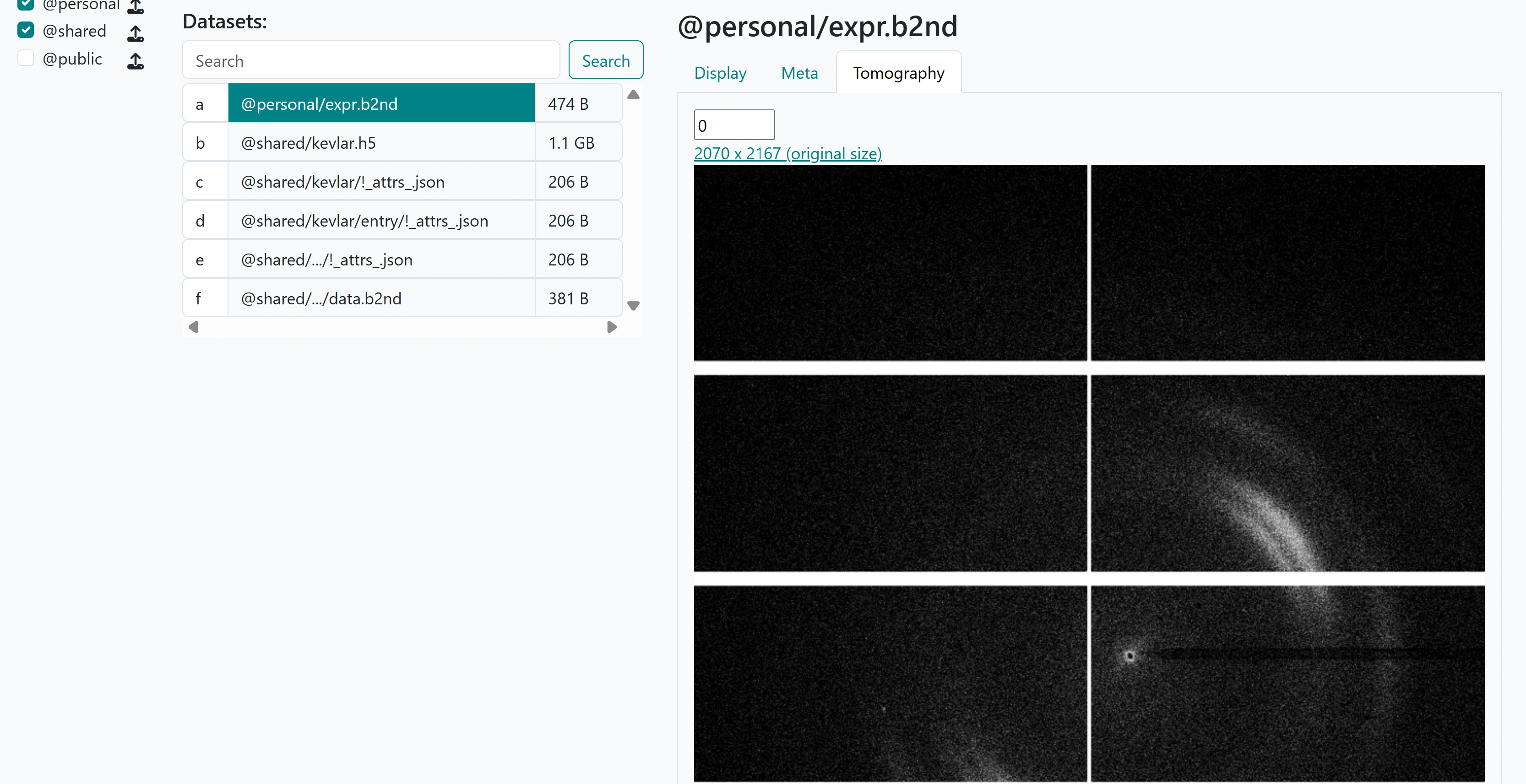
Second visualisation