Evaluating Expressions in Blosc2

What expressions are?

The forthcoming version of Blosc2 will bring a powerful tool for performing mathematical operations on pre-compressed arrays, that is, on arrays whose data has been reduced in size using compression techniques. This functionality provides a flexible and efficient way to perform a wide range of operations, such as addition, subtraction, multiplication and other mathematical functions, directly on compressed arrays. This approach saves time and resources, especially when working with large data sets.

An example of expression evaluation in Blosc2 might be:

dtype = np.float64
shape = [30_000, 4_000]
size = shape[0] * shape[1]
a = np.linspace(0, 10, num=size, dtype=dtype).reshape(shape)
b = np.linspace(0, 10, num=size, dtype=dtype).reshape(shape)
c = np.linspace(0, 10, num=size, dtype=dtype).reshape(shape)

#  Convert numpy arrays to Blosc2 arrays
a1 = blosc2.asarray(a, cparams=cparams)
b1 = blosc2.asarray(b, cparams=cparams)
c1 = blosc2.asarray(c, cparams=cparams)

# Perform the mathematical operation
expr = a1 + b1 * c1  # LazyExpr expression
expr += 2  # expressions can be modified
output = expr.eval(cparams=cparams)  # evaluate! (output is compressed too)

Compressed arrays ( a1, b1, c1) are created from existing numpy arrays ( a, b, c) using Blosc2, then mathematical operations are performed on these compressed arrays using general algebraic expressions. The evaluation of these expressions is lazy, in that they are not evaluated immediately, but are meant to be evaluated later. Finally, the resulting expression is actually evaluated (via .eval()) and the desired output (compressed as well) is obtained.

How it works

Split operands in chunks

Blosc2 uses a strategy called "blocking", which divides large data sets into small pieces called "chunks". These blocks are typically small enough to fit into the cache memory of modern processors. By working within the cache memory, Blosc2 can compress and decompress data very quickly, as it avoids the comparatively large waiting times associated with accessing main memory.

In addition, Blosc2 also takes advantage of other features of modern processors, such as SIMD (SSE2), which is a way for processors to perform multiple calculations in parallel, by using multiple cores.

Evaluate the expressions for the chunks

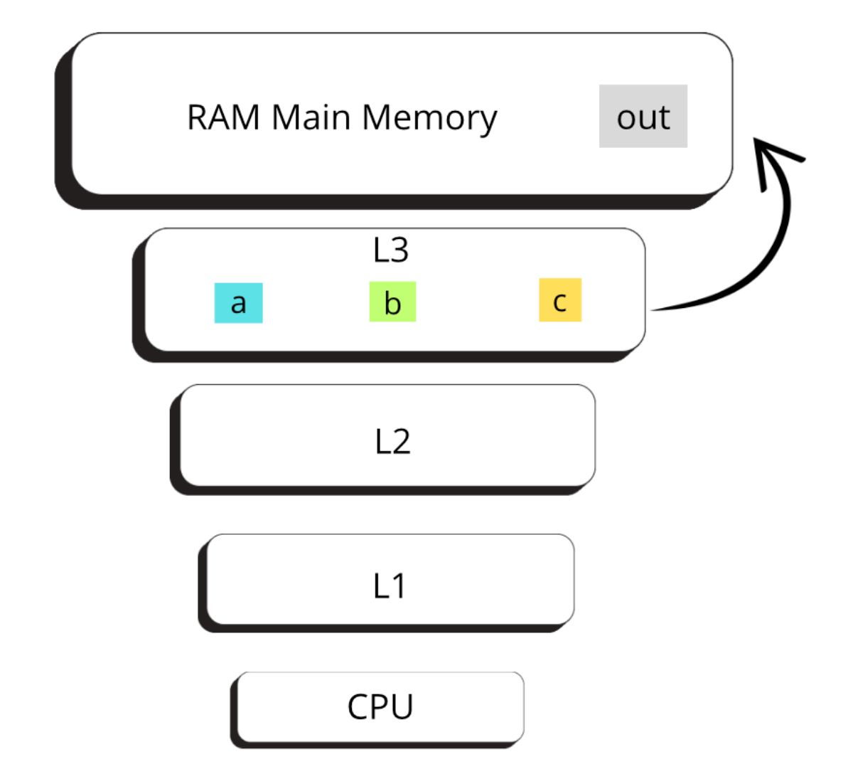
Cache hierarchies are essential components in the architecture of modern processors. They are designed to improve system performance by reducing data access times and minimizing latency in the transfer of information between main memory and the CPU.

Blosc2 employs the "divide and conquer" strategy to handle large data sets efficiently. First, it divides the data into smaller chunks using the blocking technique. Then, it evaluates the expressions in each of these chunks individually. This involves performing compression or decompression operations on each block of data separately. By breaking the problem into more manageable chunks, Blosc2 can take full advantage memory hierarchy, resulting in faster and more efficient data processing.

Store the partial result

Once the array has been divided into chunks, the operators are strategically stored in the L3 cache. This cache, shared between the CPU cores, provides fast access to data when required for operations such as data compression or decompression.

After processing the chunks of operands stored in the L3 cache (arrays a, b and c), the results of the evaluation are stored in main memory (output) . Although the main memory is slower than the cache, it provides substantially more capacity for storing data, ensuring that the results can be stored efficiently for future use.

Making the most out of the evaluation speed

In this section we will examine two plots that illustrate the performance of our system for different configurations. Our goal is to evaluate how we can optimize our resources to achieve maximum performance.

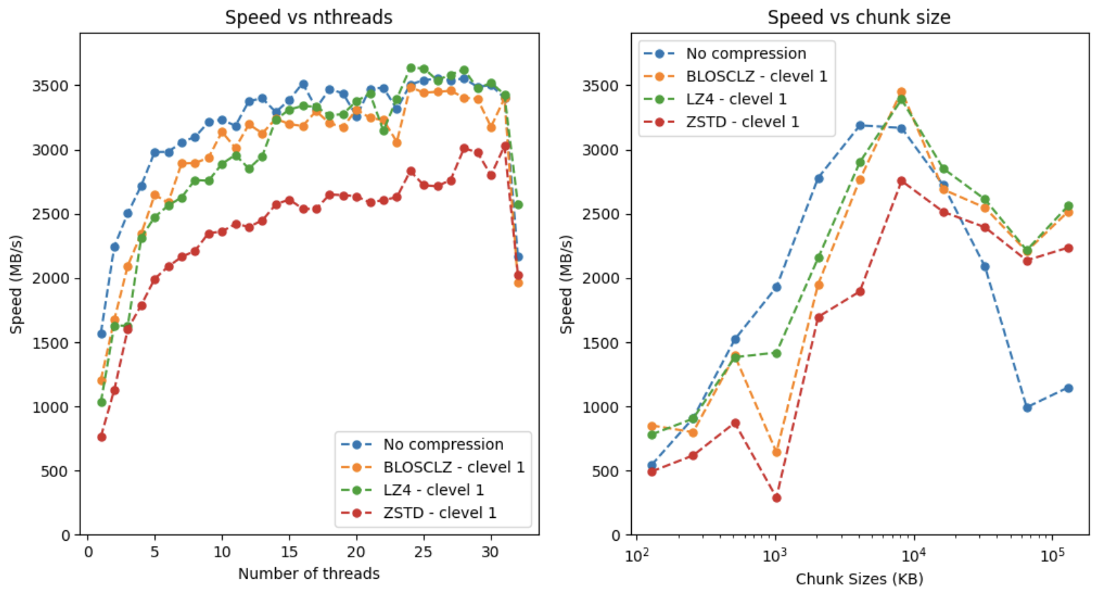
The above plots provide a detailed view of the evaluation speed when using different parameters during the evaluation of our lazy expression. Different compression codecs (using BLOSCLZ, LZ4 and ZSTD internal codecs here) affect not only how data is reduced in size, but also speed-wise. Moreover, different thread counts and chunk sizes are explored to identify performance patterns. Note that we are interested in making the evaluation as fast as possible, so we won't worry at compression ratios here.

As for the first plot, the program evaluate expressions with different compression codecs and number of processing threads (up to 32 threads, the maximum logical cores in our CPU). The objective is to measure and compare the execution times with each combination of compression configuration and number of threads. In this case the size of the data chunks is set to 8 MB (which offers pretty good performance for all explored cases).

We observe that without compression the maximum performance is reached with 16 threads, while with compression the maximum is reached with 24 threads and beyond. This is because handling less data reduces the competition for resources.

Also, note how ZSTD with clevel=1 offers a good balance between speed and compression. This is not quite a coincidence, as this combination strikes and excellent balance in general; no wonder this is the default codec and compression level in Python-Blosc2.

Experimenting with chunk sizes

It is important to recognize that there is no single or universal solution. Instead, the user may have to actively perform experiments to find the most appropriate configuration that maximizes the performance of their system based while fulfilling their requirements and constraints.

The second plot presents performance tests for the evaluation with different chunk sizes. In this case we have set the number of threads to 28; as we have seen before, this figure represents a nice balance between non-compression and compression performance.

In the plot, we observe a point where the speed reaches its maximum when the chunk size is 8 MB. In our case, we have three operators (a1, b1, c1), so the L3 cache will store the three operators and the output (8 MB * 3 + 8 MB = 32 MB), which is less than the L3 in our CPU (36 MB). When this point is reached, the speed with compression and without compression is very close. This is due to the efficient use of the level 3 (L3) cache, which acts as a shared buffer between CPU cores. The result is a significant reduction in data access times for the compressed scenario, and thus an increase in processing speed.

Finally, we note that when the chunk size is beyond 8 MB, the performance decreases. This is because, once the L3 capacity is exceeded, data needs to travel to memory more often. In this situation, when the data is compressed, less data is sent to memory and hence the speed is higher. On the other hand, when the data is uncompressed, more data is sent to memory, leading to more competition for resources and, as a consequence, we see a decrease in speed. In other words, for large chunk sizes (exceeding the size of L3), better performance is obtained with compression.

This analysis highlights the importance of choosing the right parameters (number of threads, chunk sizes, codecs, compression levels) that makes the operands to fit in L3 cache for achieving good performance.

What I’ve learned

During my internship, I immersed myself in the Big Data development environment, exploring key tools for efficient manipulation of large datasets, such as NumPy, Blosc2, and how to evaluate algebraic expressions using the later.

Discovering the direct impact of cache hierarchies and data organization optimization on system performance was particularly interesting. However, dealing with the different compression codecs, compression levels, number of threads and chunk sizes requires a careful approach and a thorough understanding of the underlying concepts.

This experience allowed me to improve my technical skills and develop a deeper appreciation of the complexity of big data processing and computing.