Caterva2 Agent: A Companion for Scientific Dataset Exploration

Scientific datasets are powerful, but exploring them can be tricky and time-consuming. You write boilerplate to list datasets, remember specific syntax, switch mental models between server-side APIs and local operations, and pray you don't accidentally load 50GB into RAM.
That's why we built the Caterva2 Agent — not as a replacement for the analyst, but as a companion that removes the busywork standing between your data and your insight. The core idea is simple: you ask for what you need in natural language, and the agent grounds every answer in real tool calls against the actual data. No hallucinated statistics. No made-up shapes. Every number, every slice, every plot comes from executing real operations on real datasets.
But here's what makes it genuinely useful for scientific work: the agent is designed to sit inside your existing Jupyter notebook exploration workflow, not replace it. You can start from the server, fetch a useful subset, work locally in your notebook with your own transformations, and then continue with the agent from that exact point, since it can see your variables and use them, and you can run your own code on the agent's responses. It's a loop: agent-assisted exploration → manual analysis → agent-assisted exploration, seamlessly switching between server-side operations and local ones as you go.
A short demo of the Caterva2 Agent in action.
How It Works: Architecture and Operations
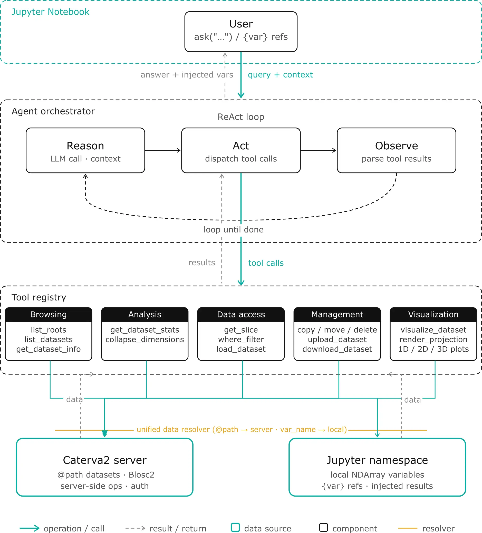
Let's look at what the agent actually does and how it's structured. The architecture is built around three layers: the LLM orchestrator (the reasoning brain), the tool layer (the hands that manipulate data), and the data bridge (the connection between server, local memory, and your notebook).
The Notebook Bridge: User-Agent Collaboration
The agent isn't a black box you send requests to and receive answers from. It lives inside your Jupyter notebook and shares the same Python namespace as you. This means the collaboration is bidirectional: you can see and operate on everything the agent does, and the agent can see and operate on everything you do.
When the agent fetches a dataset from the server, it doesn't just return a text summary — it injects the actual array into your notebook as a variable you can use immediately. Ask for a slice of @public/examples/temperature.b2nd, and temperature appears in your namespace. Run your own transformations (temp_celsius = (temperature - 32) * 5/9), then hand it back to the agent with ask("Plot a histogram of {temp_celsius}"). The agent reads your temp_celsius directly from the notebook's user namespace, sees its current shape and dtype, and continues from exactly where you left off. No data copying, no context switching, no "export to CSV and re-import."
The notebook interface provides the commands for this workflow: ask(message) sends questions and injects results, variables() lists what the agent has created, clear_variables() cleans up without losing conversation history, and login() / logout() manage server authentication. The {variable} syntax is the bridge — when you reference {my_data}, the agent expands it to include metadata (shape, dtype, statistics) in its prompt before deciding which tools to call.
Under the hood, this works through a simple registry pattern. When tools fetch server data, they register results in an internal _fetched_objects dictionary. After the agent finishes reasoning, ask() retrieves from this registry, sanitizes names to valid Python identifiers, and injects them into your notebook's user namespace. For local references, the agent looks up {var_name} in the notebook namespace, validates it's array-like, and prepends that context to your message. The loop is seamless: you work with the agent, then independently, then with the agent again — all within the same conversation and the same namespace.
The Unified Data Model: One Interface, Two Sources
The most important architectural decision is the unified resolver. Every tool that operates on data uses the same resolution logic:
- Path starts with
@→ Server dataset. The agent creates a Caterva2 client (authenticated if you've calledlogin()), fetches the dataset handle, and operates on it server-side. - Otherwise → Local notebook variable. The agent reads from the notebook namespace, validates that the object is array-like (has
shapeanddtype), normalizes it toblosc2.NDArraywhen possible, and operates on it locally.
This means get_dataset_stats("@public/data.b2nd") and get_dataset_stats("my_local_array") use the exact same code path. The tool doesn't know or care where the data comes from — it sees a unified ResolvedData object with .shape, .dtype, and [] accessor. This is what enables the seamless switching between server and local operations in your workflow.
The Five Tool Families
The agent exposes 15 tools organized into five categories. Each tool is defined by a JSON schema (description, parameters, types, enums) that the LLM uses to decide when and how to call it.
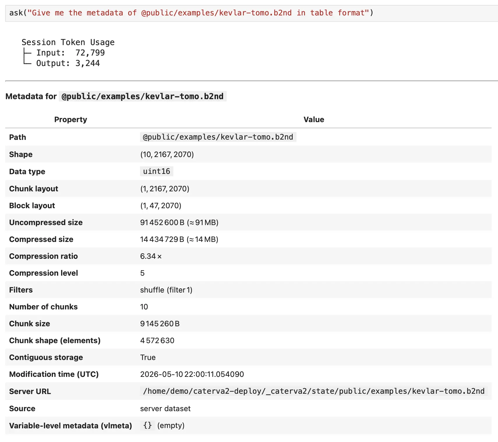
Browsing tools handle discovery. list_roots shows top-level collections (@public, @personal, @shared). list_datasets("@public/examples") paginates through items in a path. get_dataset_info("@public/examples/ds-3d.b2nd") returns full metadata: shape, dtype, chunk layout, compression codec, ratio, and timestamps. These tools answer "what do I have?" before you touch any data.
Analysis tools compute on the data. get_dataset_stats calculates min, max, mean, std, var, argmin, argmax, any, and all — either globally or along a specific axis. collapse_dimensions is the heavy lifter for large datasets: it reduces N-D to (N-1)-D via aggregation (max, mean, sum, min, std, var, prod) executed server-side on compressed Blosc2 chunks without downloading the full array, or on local variables if desired. For a 3D tomography, collapse_dimensions(path, axis=0, operation="max") gives you a 2D max-intensity projection in seconds.
Data access tools retrieve values. get_slice parses Python-style slice strings ("0:100", "0:5, 0:3", ":, 0") and returns the data. For large slices (>100 elements), it returns a summary (shape, min, max, mean, preview) instead of dumping the full array into the conversation. You can persist sliced results to @personal/slices/... for follow-up operations. where_filter applies conditional selection (elevation > 3000) and returns value_if_true where the condition is met, and value_if_false elsewhere. It auto-saves to @personal/where_filter/... when authenticated with the Caterva2 server. load_dataset, does exactly what it sounds like: it loads datasets from the server into the notebook locally.
Dataset management tools handle server-side file operations. copy_dataset, move_dataset, and remove_dataset require authentication. Move and remove need explicit confirmation to the agent to execute — this prevents accidental data loss. upload_dataset takes a local variable and pushes it to @personal/... as a Blosc2 array. download_dataset returns a direct URL for external download.
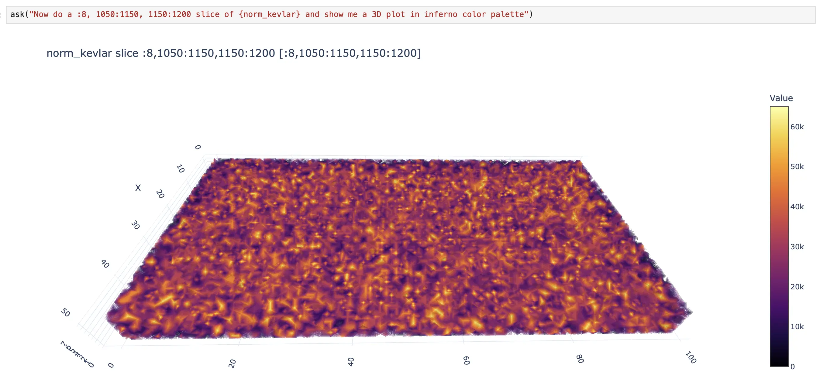
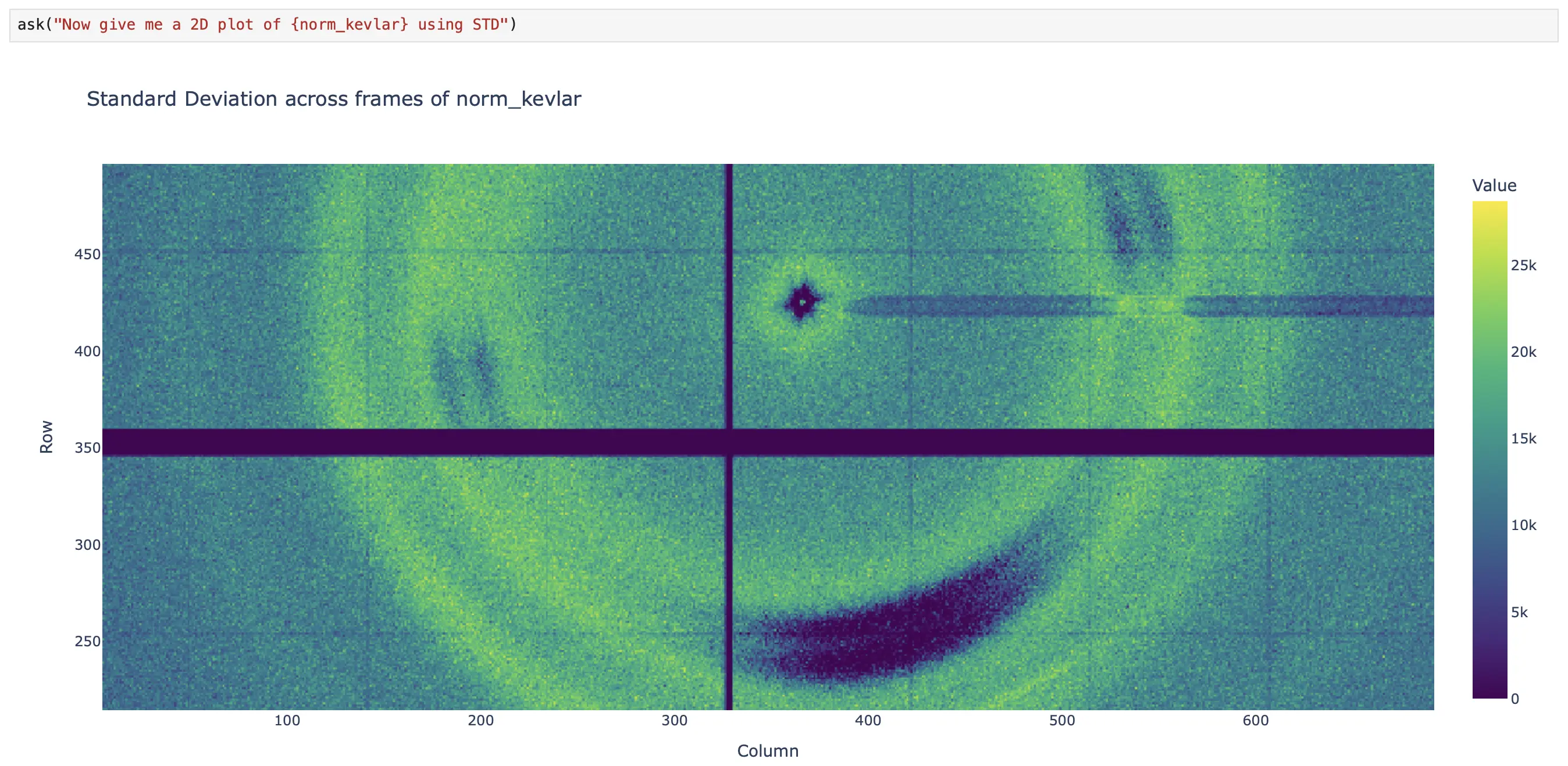
Visualization tools render what you see. visualize_dataset auto-detects dimensionality and creates interactive Plotly plots: 1D line plots, 2D heatmaps with equal aspect ratio, 3D volume rendering with adjustable opacity. Large datasets are automatically downsampled. For giant data that exceeds interactive limits, render_projection first collapses dimensions, then downsamples to 2000×2000 pixels, and returns a base64-encoded PNG — ideal for multi-GB datasets where interactive rendering would be impossible.
Chaining Operations: The Power of Persistence
The real power emerges when you chain these tools together. Because derived results can be persisted back to the server (under @personal/) or injected into your notebook namespace, subsequent operations can continue from exactly where you left off.
Server-side chaining example:
# Filter a massive elevation dataset
ask("Filter @public/large/survey.b2nd where elevation > 3000")
# → Result persisted to @personal/where_filter/survey_elevation_20240115T120000.b2nd

# Collapse the filtered result without downloading it
ask("Collapse the previous result along axis 0 with mean")
# → Operates on the @personal path directly, returns @personal/collapsed/...

# Visualize the 2D projection
ask("Render a static projection of the collapsed data")
# → Server-side 2D PNG, never touches local RAM with the full dataset
Local chaining example:
# Fetch a slice
ask("Get slice 0:100 from @public/examples/temperature.b2nd and load it locally")
# → Injects temperature into namespace

# Manual transformation
temp_celsius = (temperature - 32) * 5/9

# Continue with agent using the local variable
ask("Compute stats on {temp_celsius}")
# → Agent sees temp_celsius, operates locally, returns statistics
The agent remembers which operations produced server-side results and which produced local variables. Server results return result_path hints for follow-up server calls. Local results get unique variable names injected into your namespace. The loop is seamless: server → local → server → local, all within the same conversation.
What This Looks Like in Practice
Let me walk you through a simple but realistic workflow:
A simple but realistic workflow of Caterva2 Agent in action.
Notice how, at some point, the user and the agent begin alternating responsibilities. The agent handles the boilerplate tasks (listing datasets, fetching data, retrieving metadata). The user handles the domain-specific reasoning, such as scaling the dataset values to address the dynamic-range visualization problem (norm_kevlar = blosc2.clip(sliced_kevlar_tomo, 0, 5) * 13000). Then the agent takes over again for the visualization. This is the collaborative loop in action.
Conclusion
The Caterva2 Agent was built to remove the busywork from scientific dataset exploration. By combining a ReAct-style loop with a unified server/local data model, it acts as a collaborative companion that handles the boilerplate — listing datasets, slicing arrays, filtering data, plotting results — while leaving the domain-specific reasoning to you.
It lives directly inside your Jupyter notebook, shares your namespace, and hands control back whenever you want to apply your own expertise or modify the workflow manually. Under the hood, it uses unified dataset resolution for seamless server/local switching, Blosc2-first execution for high-performance data handling, and strict guardrails to keep operations safe and predictable.
If you work with NDArray Blosc2 datasets — whether hosted on a Caterva2 server or stored locally — the goal is simple: make exploration faster, smoother, and genuinely collaborative.